


01 / Origin
Start where the cargo is.
The marked origins identify the production areas in the example. The soybean view puts both paths from Mato Grosso on the same plate.
01 / Brazilian commodity intelligence
One to the port. One into the price. KAIRO brings forward export basis and logistics risk into the same view for desks trading Brazilian commodities.
Follow a hypothetical soybean cargo from Mato Grosso. The atlas starts with the choice of gateway and ends with the record a desk can review.
02 / Brazil in world trade
Whole soybeans and corn, the products of soybean crushing, raw cane sugar and iron ore connect Brazil to several global commodity markets. The trade figures show the scale of the flows behind the choice of cargo, gateway and delivery window.
Photographic plate / Six covered markets
Brazilian exports · Calendar year 2025 · Million metric tonnes
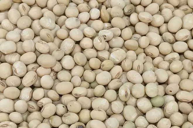
Specimen 01
108.2 Mt
Soybeans other than seed

Specimen 02
40.9 Mt
Corn grain other than seed
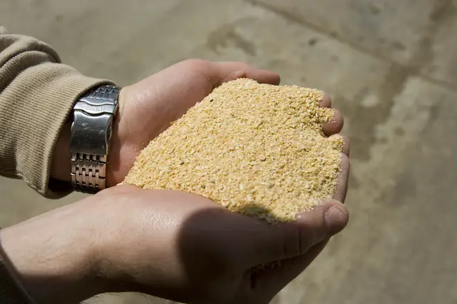
Specimen 03
23.3 Mt
Meal and other solid extraction residues

Specimen 04
1.3 Mt
Crude soybean oil, including degummed oil

Specimen 05
29.5 Mt
Broader raw cane sugar category used for context
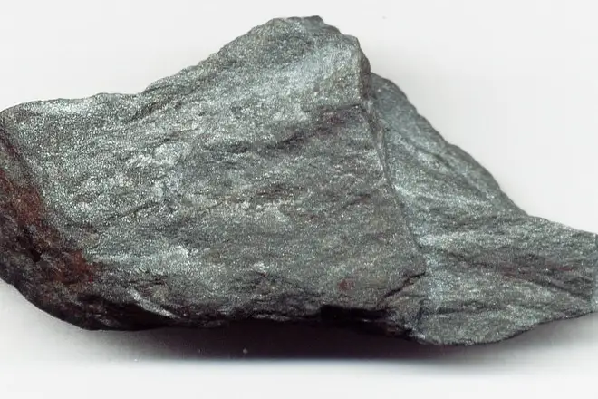
Specimen 06
392.4 Mt
Non-agglomerated iron ore and concentrates
Net export weight for the selected customs categories, rounded to one decimal place. The raw cane sugar category covers a broader market than the VHP grade. The photographs illustrate the commodities. Source · SECEX / Comex Stat
Photographs cropped and resized for this plate.
03 / Market thesis
Take a hypothetical soybean cargo in Mato Grosso. Sending it north to Barcarena or south to Santos gives the desk two different delivery exposures.
National balance sheets frame the crop year. The desk still has to choose a gateway and a delivery window, while other commodities may be seeking capacity at the same port.
The commercial choice
The map locates the gateways and shows where the comparison starts. Follow the cargo on the map ↓
Illustrative export chain. The inland route and transport mode depend on the corridor.
04 / Export corridors
Follow the soybean routes from Mato Grosso to Barcarena and Santos. Switch to corn to see how a different origin and gateway change which corridor a desk needs to watch.
Figure 01 / Illustrative
Soybeans · Mato Grosso to Barcarena and Santos, and Rio Grande do Sul to Rio Grande.
Lines and motion show direction schematically. Boundary source.
A visual key to transport modes. The route lines on the map show direction.
01 / Origin
The marked origins identify the production areas in the example. The soybean view puts both paths from Mato Grosso on the same plate.
02 / Gateway
The animation shows direction. The lines are schematic and carry no volume, journey time or live vessel information.
03 / Comparison
With the gateways in view, compare quotes for the same commodity, delivery window and unit.
05 / Forward basis
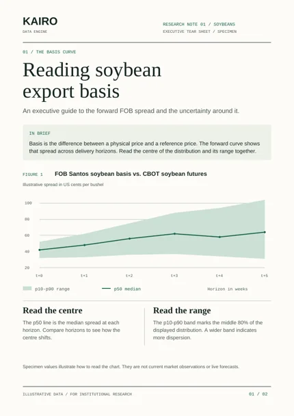
Suppose the cargo goes to Santos. Export basis is the difference between the physical FOB price and its reference benchmark. Select a horizon to see how that spread and its range change across delivery windows.
The curve uses illustrative soybean values in US cents per bushel.
Figure 02 / Illustrative
US ¢/bu
Central estimate
P50 is the midpoint of the distribution for that delivery horizon. The example moves from 47 at T+0 to 70 at T+5.
Range of outcomes
P10 and P90 bound the central 80% of the distribution. The example widens from 41–54 at T+0 to 41–100 at T+5.
Comparability
When comparing delivery windows, hold the commodity, gateway, benchmark and unit constant so the change reflects the horizon.
06 / Reading the signals
Once the desk has the curve in front of it, the next step is to put the price range alongside the timing and location of the exposure.
01 / Price
A later window in the Santos example has a higher median and a wider band. Examine both before deciding which window deserves more work.
02 / Timing
Read the logistics regime alongside the forward curve and snapshot date. Then check the delivery window against the desk’s physical commitments.
03 / Location
Compare the indicators for the relevant gateways on the same cutoff. Review whether the freight and delivery assumptions still hold for each route.
Worked reading. At T+5, the illustrative Santos median rises by 23¢/bu while the lower quantile stays at 41¢/bu. A desk can use that difference to frame a question about the later window, then check logistics and quote terms before drawing a conclusion.
07 / Institutional use cases
Five ways institutional desks can use forward basis and Brazilian commodity logistics signals to research potential sources of alpha, stress-test exposures and decide what to investigate next.
01 / Macro
02 / Systematic
03 / Physical
04 / Equities
RAIL3).05 / Credit
Field plates / Illustrative data
01 / Forward basis
Illustrative soybean basis in US cents per bushel.
P10–P90━ P50 median
02 / API snapshot
Illustrative excerpt from the public response contract.
{
  "commodity": "SOYBEANS",
  "market_regime": "ELEVATED_LOGISTIC_PRESSURE",
  "corridors": [
    {
      "corridor_id": "SANTOS",
      "saturation_probability": 0.62,
      "freight_pressure_index": 74
    }
  ]
}
Read the API response contract. Throughput is illustrated separately below.
03 / Export corridors
Illustrative throughput as a share of capacity, with example status labels.
04 / Executive tear sheet
Illustrative report spread with a physical balance and a corridor chart.
01 / Physical balance
| Opening stock | 2.0 |
|---|---|
| Receipts | 8.0 |
| Shipments | 6.4 |
| Closing stock | 3.6 |
02 / Corridor capacity
Illustrative throughput / capacity
08 / Institutional products
Take the same basis and logistics view into a meeting or bring the dated snapshot into a research workflow.
01 / Macro PMs & trading desks
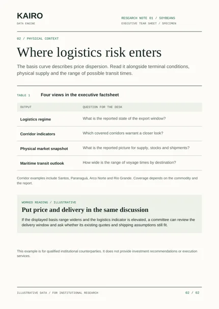
A two-page research note for a meeting or a handover between desks. Read the two pages together to connect the forward spread with the physical market.
Soybeans · Two pages · Illustrative data
02 / Quants, CTAs & systematic desks
Bring delivery horizons, basis quantiles and logistics indicators into a desk workflow. Keep the cutoff and provenance fields with each stored snapshot.
GET /v1/signals/SOYBEANS/latest
Open API reference ↗
09 / Coverage
The atlas follows soybeans. The feed also covers corn, soybean products, VHP sugar and iron ore. Use the commodity identifiers below when inspecting the API.
SOYBEANSCORNSOY_MEALSOY_OILSUGARIRON_ORE10 / Market dispatches
Source-linked news from Brazil’s commodity markets. Each edition brings together developments in crops, processing, minerals, trade and freight.
KAIRO / Public sources
No market brief has been published yet.
11 / Research evidence
Review the product’s presentation, the fields the API returns and the evidence a desk would need before relying on the signal.
12 / Research and models
Customs records show what was shipped. Crop releases, port activity and freight indicators put those volumes in context. Econometric models offer one way to test whether a signal adds information against a clear reference.
Validation and catalogue coverage
A / Empirical retrospective validation (2023–2024)
A 24-month retrospective comparison for national export volumes. Models were held fixed for January 2023 to December 2024 after fitting to historical series from January 2014 through December 2022. Evaluated against the standard institutional benchmark: Seasonal Naïve (t−12).
01 / Retrospective benchmark
Monthly net export weight · 2023–2024 · Million metric tonnes (Mt)
H1 Harvest Peak. Soybeans peak between March and May. 20 of 24 months fall strictly inside the empirical 80% error dispersion band.
02 / Retrospective benchmark
Monthly net export weight · 2023–2024 · Million metric tonnes (Mt)
H2 Safrinha Ramp. Corn shipments peak between August and October, providing a counter-cyclical balance to soybean logistics at export terminals.
03 / Error comparison · Soybeans
Out-of-sample models on 2023–2024 (24 months) against the seasonal baseline.
The enriched model delivers a 57.8% lower MAE vs. Seasonal Naïve (+13.1% gain over baseline) across the 24 retrospective test months.
04 / Error comparison · Corn
Corn out-of-sample models on 2023–2024 (24 months) against the seasonal baseline.
The corn model achieves a 55.4% lower MAE vs. Seasonal Naïve, capturing both low-water river draft restrictions and rail redirections.
05 / Port logistics risk benchmark
Monthly lineup waiting days · 2024 calendar year · Days per vessel
Harvest Demurrage Surcharge. Congestion spikes in Q2 create demurrage costs of ~$25,000/day, directly modulating forward FOB export basis differentials.
06 / National throughput distribution
13.45 million metric tonnes reconciled across 22 port facilities in peak month.
Reconciled directly against official ANTAQ microdata with cryptographic receipt verification.
B / Multi-commodity catalogue & taxonomy of evidence
KAIRO classifies empirical evidence under a four-level governance framework. Grains (soybeans and corn) feature audited retrospective evaluations with high-frequency proxies. Derivatives and iron ore operate under zero-leakage physical capacity simulations (lineup_weight = 0.0).
| Commodity | Research status | Audited metrics & monitoring scope |
|---|---|---|
| Soybeans | Retrospective (Proxies) | Retrospective 2023–2024: Enriched MAE = 0.762 Mt (−57.8% vs. Naïve 1.808 Mt), Pearson r = 0.9776, Rank-IC = 0.9583 (t = 15.72), Hit Ratio = 87.0%. Port rain stoppages and silo pace proxies. |
| Corn | Retrospective (Proxies) | Retrospective 2023–2024: Enriched MAE = 0.578 Mt (−55.4% vs. Naïve 1.295 Mt), Pearson r = 0.9684, Rank-IC = 0.9574 (t = 15.53), Hit Ratio = 78.3% (82.6% turning points). Northern Arc waterway draft drops and rail redirection proxies. |
| VHP Sugar | Conditioned Simulation | Conditional simulation. Models berth rain closures and mill crushing pace in Santos and Paranaguá. |
| Soybean meal | Conditioned Simulation | Conditional simulation. Models industrial crush balance (1 t soy → 77.5% meal) and domestic feed absorption. |
| Soybean oil | Conditioned Simulation | Conditional simulation. Models extraction yields (19.5%), port tankage and ANP mandatory biodiesel blending (B14). |
| Iron ore | Conditioned Simulation | Conditional simulation. Models Carajás (Ponta da Madeira) & Southeastern mining corridors (Tubarão), monsoon seasonality and Capesize loading. |
C / Portfolio risk research
The API includes an illustrative breakdown of portfolio risk. Empirically calibrated factor results are unavailable.
D / Logistics scenarios
Explore how port rain, shallow waterways or rail outages could affect logistics. Results are conditional model estimates.
E / Interactive Desk Sandbox · On-Demand Stress Testing
Change the assumptions below to compare illustrative cargo flows, waiting times, demurrage and basis. The calculator uses a fixed reference case.
Stressed Corridor Throughput Reallocation (Peak Harvest Month)
13 / Signal quality
Quality has two parts. A desk needs to know what information was available at decision time, and whether the signal holds up against what actually happened.
01 / Against observed outcomes
14 / Data governance
A desk reviewing an earlier decision needs both the information cutoff and the time the snapshot became available. Preserve those fields with the record you received.
as_of_date As-of datepublished_at Publication timeprovenance_hash Provenance hashHistorical review. For a decision at a known timestamp, check when the snapshot was published before using it. Store the provenance hash with the record so the version can be referenced later.
15 / Institutional access
Start with the material that fits the review. A desk can read the public specimen and inspect the API contract before using authenticated snapshots or current reports.
Research review
Pick a commodity and delivery window. Use the two-page format to check whether it supports the questions the desk wants to ask.
See the public specimen ↑Technical review
Read the endpoint and response example. Access to current snapshots and reports requires a key issued to your institution.
Review access requirements ↗